Inside NanoChat: How 561 Million Parameters Come Together in a Transformer
Introduction
Modern language models are defined by a single number — their parameter count. Yet, behind that number lies a web of architectural design decisions that shape how the model learns, scales, and performs. In this post, we’ll take apart NanoChat d20, a compact transformer model with ≈561 M parameters, and understand exactly where each parameter comes from — from token embeddings to feed-forward layers — and how this design fits within modern scaling laws.
In large-language models (LLMs), the number of trainable parameters is more than just a statistic — it captures how much capacity the model has, how much compute and data you'll need, and what kind of tasks it can handle. In this post, we take a detailed look at the configuration and parameter-count of the NanoChat d20 model (≈561 M parameters) and explain exactly how that number is calculated, why the architectural choices were made, and how it connects to the amount of training data required. Whether you're a researcher building your own transformer from scratch or a trained-engineer tuning an off-the-shelf model, understanding these mechanics gives you a clearer view of the trade-offs involved.
Model Specifications
The d20 model is defined by these configuration parameters:
| Parameter | Value |
|---|---|
| Vocab size | 65,536 |
| Number of layers | 20 |
| Model dimension (hidden size) | 1,280 |
| Number of attention heads | 10 |
| KV heads | 10 |
From these specs, we can calculate the exact parameter count.
.png)
Parameter Calculation Breakdown
1. Embedding Layer: ~83.9M Parameters
The embedding layer maps each of the vocab tokens into a dense vector of dimension 1,280. Given a vocabulary of 65,536 tokens, we compute:
embedding_params = vocab_size × model_dim
                  = 65,536 × 1,280
                  = 83,886,080
This lookup table is essentially a matrix of size (65,536 × 1,280). One subtlety: many models tie the input-token embedding matrix with the output-projection (LM head) matrix, which would reduce total parameters. In the NanoChat d20 design, the output head is separate, so we account for both layers independently.
Why vocab size 65,536? This size (2¹⁶) gives a large enough token-set to handle rich sub-word encoding (e.g., Byte-Pair Encoding or SentencePiece) while keeping embedding lookup cost manageable. A larger vocab increases memory and parameters; smaller vocab may increase sequence length or reduce expressivity.
2. Attention Layers: ~131M Parameters
Each transformer layer contains self-attention with four projection matrices:
Per attention layer:
Query projection:    1,280 × 1,280 = 1,638,400
Key projection:      1,280 × 1,280 = 1,638,400
Value projection:    1,280 × 1,280 = 1,638,400
Output projection:   1,280 × 1,280 = 1,638,400
                                      ──────────
Total per layer:                      6,553,600
Across all 20 layers:
6,553,600 × 20 = 131,072,000 parameters3. Feed-Forward Networks: ~262M Parameters
Each layer has a 2-layer MLP with a 4× expansion ratio:
Per feed-forward layer:
Dense 1:  1,280 × 5,120 = 6,553,600
Dense 2:  5,120 × 1,280 = 6,553,600
                          ──────────
Total per layer:         13,107,200
Across all 20 layers:
13,107,200 × 20 = 262,144,000 parameters4. Layer Normalization: ~102K Parameters
Each layer has 2 layer norm operations (before attention and before FFN):
Per layer norm = scale (1,280) + bias (1,280) = 2,560
Per layer = 2 × 2,560 = 5,120
Across 20 layers = 5,120 × 20 = 102,400 parameters
5. Output/LM Head: ~83.9M Parameters
The final layer projects from model_dim back to vocab_size for next-token prediction:
Output head = model_dim × vocab_size
= 1,280 × 65,536
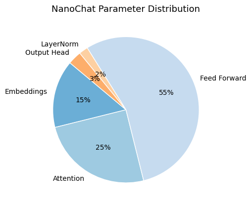
= 83,886,080 parametersTotal Parameter Count
Embedding layer:      83,886,080
Attention layers:    131,072,000
Feed-forward layers: 262,144,000
Layer normalization:    102,400
Output/LM head:       83,886,080
                     ──────────────
Total:        ≈ 561,000,000 parameters
Official count: 560,988,160 parameters (minor differences due to rounding and bias terms)
Architectural Design Choices
These specs weren't arbitrary. Here's the reasoning:
Number of Layers (20): More layers enable deeper reasoning and pattern recognition at different abstraction levels.
Model Dimension (1,280): Wider layers mean more parameters per layer, increasing model capacity.
Attention Heads (10): Distributed attention across multiple representation subspaces.
Head dimension = model_dim / num_heads = 1,280 / 10 = 128 dimensions per head128 dimensions per head is the industry standard (used in GPT, BERT, etc.).
The Chinchilla Scaling Law
DeepMind's Chinchilla paper showed that for compute-optimal performance, the total number of training tokens should be about 20 × the number of parameters.
For NanoChat:
tokens = 20 × 561M ≈ 11.2 BThat's roughly 40–50 GB of cleaned text (depending on compression).
Too few tokens → underfit model (memorises training data).
Too many tokens → waste of compute (no extra accuracy).
This ratio provides a practical rule for balancing training cost and dataset size.
Memory Footprint
Memory footprint = parameters × bytes per param.
Example for FP32, FP16, quantized:
Memory Estimate

561M × 4 bytes (FP32) = 2.24 GB
561M × 2 bytes (FP16) = 1.12 GB
561M × 1 byte (INT8) = 0.56 GB
So NanoChat can easily fit on a single consumer GPU (like an RTX 3090 24 GB) with room for batch processing.
Model Comparison
| Model | Params | Memory (FP16) | Optimal Tokens (B) |
|---|---|---|---|
| NanoChat d20 | 0.56 B | 1.1 GB | 11 B |
| GPT-2 Medium | 0.35 B | 0.7 GB | 7 B |
| Llama-2-7B | 7 B | 14 GB | 140 B |
From Parameters to Training Data
This determines the dataset size:
Assuming 4.8 characters per token:
Total characters = 11.2B tokens × 4.8 = 53.76B characters

At 250M characters per shard:
Shards needed = 53.76B ÷ 250M ≈ 215 shards → rounded to 240 shards

Total disk space = 240 shards × 100MB = ~24GB
Key Takeaways
- Parameters emerge from architecture choices — We design the specs, then calculate parameters
- Standard ratios exist — 10 attention heads with 128 dims per head is optimal
- Scaling is predictable — Chinchilla law connects parameters to training data
- Every component contributes — Embeddings, attention, and FFN layers are all significant
The Full Pipeline
Architecture Specs → Calculate Parameters → Apply Chinchilla Law → Determine Data Needs
    (20, 1280)    →    (561M params)    →   (11.2B tokens)     →  (240 shards, 24GB)
This systematic approach ensures the model is trained with optimal compute allocation—not underfitting from too little data, nor wasting compute on excess data.